A reproducible workflow with Jupyter on Chameleon
- Oct. 25, 2019 by
- Jason Anderson
Jupyter notebooks are a great tool for structuring your computer science experiments on Chameleon because they allow you to iterate on your idea interactively, intuitively, and quickly. But, it may not be obvious how you can leverage this tool for running an experiment, especially if you are used to thinking of Jupyter notebooks as purely tools for crunching and analyzing data or producing rich visualizations.
In this post, we’ll show you how to take a sample experiment--in our case, one measuring the impact of CPU utilization on a bare metal node’s power usage--and break it down such that we can reliably reproduce it via a Jupyter notebook. We’ll take advantage of Chameleon’s powerful Jupyter environment, where the testbed is integrated such that you can reserve resources and provision nodes without leaving the Notebook. But beyond that, we’ll show how you can “drive” your experiment remotely all within Jupyter, a simple idea that nonetheless significantly simplifies documenting and developing your process as you explore. Hopefully you will leave with some ideas about how to leverage this functionality in your future experimentation to make your process more streamlined, reliable, and shareable.
First, if you haven’t already tried it out, head on over to Jupyter on Chameleon and log in with your Chameleon credentials; a new Jupyter Notebook server will be automatically provisioned for you. If you followed that link, you’ll automatically have our example opened for you; if not, you can find it at “notebooks/examples/power-experiment/RunExperiment.ipynb” in your Jupyter Notebook server.
Step 1: defining your environment
This example starts with a bit of code that points the Notebook to an actual bare metal node provisioned by Chameleon. For this example, we assume that you’ve already provisioned a bare metal node, perhaps via another tutorial. In the Notebook you can plug in the Floating IP of your instance; as long as your node’s SSH keypair is stored within the Jupyter server (this is done for you if you followed the tutorial for provisioning a node via the CLI), you’ll be able to access your node just fine directly from Jupyter. This is nice, as it allows you to come back days or weeks later and simply plug in a new IP at the top of the Notebook; the rest of the Notebook will reference this variable and will “drive” the experiment on whatever node is at this address.
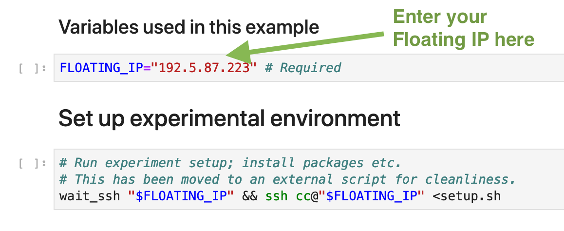
Next, we have a block of code defined that performs some setup on our node. For this power experiment, I need a new package installed on top of the base Chameleon CC-CentOS7 image (though, I could have avoided this step if I had used a disk snapshot I had setup prior). I personally find it easier to work with single-purpose scripts, so I created a `setup.sh` script in my Notebook directory. Then, in my Notebook, I simply have a step where I execute the script remotely via SSH. I can re-run this setup script if I ever make changes to the dependencies needed by the rest of my experiment. As a bonus, at the end of this, all of my dependencies are documented!
Step 2: run the experiment
This experiment simply collects power usage as measured by the node when under variable load. I have designed a little run script to launch my experiment, which consists of three stages: first I measure the power usage when stressing 24% of my CPU cores, then I measure the usage when 50% are stressed, and finally I measure when all cores are stressed. The entire experiment run is encapsulated in this `run_experiment.sh` script. Additionally, for my convenience, I enabled some primitive parameterization of the script: I can pass a few command-line args to determine how many runs I will perform, the delay between runs, and the sample rate for the power measurements.
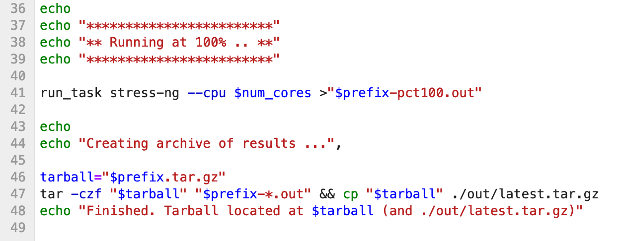
A portion of our experiment script.
To actually invoke this script, this time I copy it to the node via SCP and then invoke it locally on the node with some parameters. I can adjust the parameters in my Notebook and easily re-run with a different sample rate or number of runs. Similarly, I can edit the experiment script to change how it works and re-invoke it in the same way as before.
The script will output result data files to the node’s local disk. I want to analyze them in my Jupyter Notebook, so the last step is to copy the files back down to my Notebook directory, again via SCP. I had a few different files, so I first zipped them up in a tarball and then I extract inside the Notebook.
Step 3: analyze the results
For the analysis, I have a separate Notebook called “Analysis.ipynb”; this is due to a technical limitation whereby I can’t have both Bash and Python in one Jupyter Notebook at the moment. I want to use Python libraries like matplotlib to plot this data, so I need a Notebook that has Python enabled. Bash was very useful for running my experiment, but it’s not the right tool for this job.
My analysis is pretty simple, but it still takes a bit of processing to get these results parsed and displayed in a graph. I am using some common Python libraries like pandas and matplotlib to do the heavy-lifting. Fortunately, I only have to write this code once: I can re-run it each time I get new results to compare how things look. I can save the graphs as images to include in a publication if I wish as well.
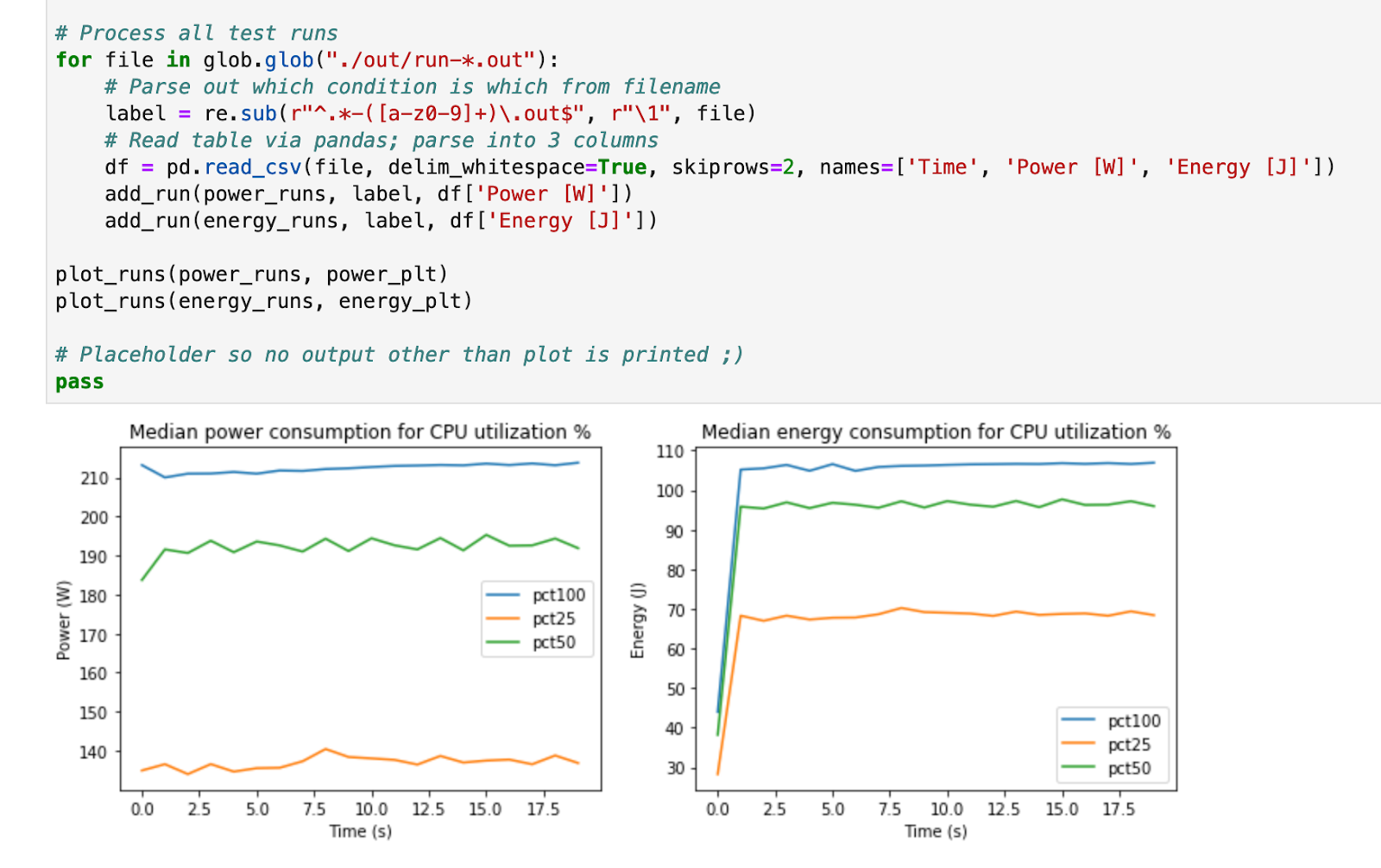
Example output from the analysis.
Next steps
This example has hopefully helped you think about how you might consider breaking your experiment into a few steps and thinking about how you can make each step easier to redo.
If you want to watch a webinar where we go over this experiment in more detail, you can find it on YouTube.
No comments